Introduction
The previous blog post, The Stonemont Quality KPI, focused on explaining the Stonemont KPI and the potential use of this value as a measurement of risk associated with aggregate products, asphalt mixes, and concrete mixes. In this blog post, we will show an example of using the KPI and the associated statistical measurements for an asphalt mix design. While the discussions here will focus on asphalt mixes, the same principals can be applied to aggregate products and concrete mixes.
Stonemont software uses the KPI and the associated statistics in several reports and analysis tools available in the program. One of these tools is “Mix Risk”, which uses the Stonemont KPI to provide an evaluation of potential future performance of a mix design prior to or during production of the mix. The Mix Risk tool is available when performing any blending of aggregates including asphalt and concrete mixes.
What is Mix Risk?
When designing an asphalt mix, you include multiple aggregate components that presumably have been sampled and therefore have a measured average gradation and variation or standard deviation. Sometimes the gradations for components used in constructing asphalt mixes are developed from a limited number of samples obtained within a short time frame. For example, a small set of samples are obtained from a source stockpile, and the average of those samples is used for the component when constructing a design. Since this is a small sample set, it may not accurately represent the average or variation of the gradation. If the variation is too small it may result in an artificial confidence in the mix. If the variation is too large, it may serve as a safety factor to the mix design but that can result in a less than ideal mix if it is changed to account for this increase in variation. When possible, it is best to use a set of samples over a longer time period that will better reflect the true average and variation of the material.
Mix Risk uses a Monte-Carlo simulation to evaluate the mix design considering the uncertainty with each of the component gradations as defined by their means and standard deviations. A Monte-Carlo simulation is a mathematical technique that relies on repeated random sampling to obtain numerical results that allow the process (producing the mix) to be simulated many times over. In Stonemont software, Mix Risk will create a set of randomly generated gradations using the mean and standard deviations for each component and combine them using the percent each is contributing to the design. The randomly generated gradations, each of which represents a plausible combination of aggregates in the mix design, are then analyzed using the Stonemont KPI.
Both the average and standard deviation values associated with the component gradations are important. The average values are used to construct a mix in an effort to reach some desired target value. However, the average value by itself doesn’t reflect the variation associated with each component gradation. Therefore the combined gradation of the mix will vary during production. Understanding how that mix may vary during production from the average design is the key benefit of a Mix Risk analysis. The results of the Mix Risk analysis will allow you to make informed decisions regarding the viability or risk of producing the mix.
Asphalt Mix Example
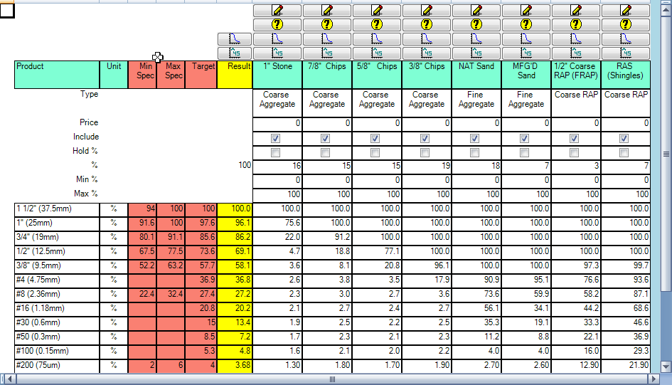
An example might lend insight into the value of using the mix risk tool. Figure 1 shows the proportions for an asphalt mix. This mix could be a new mix or it could be a mix already in production. For the purposes of this example, the aggregate components are being produced and tested at a co-located quarry that uses Stonemont Software so the data can be easily queried and updated. We are evaluating the mix to determine how the component gradations are having an effect on the mix design. The percentage of each component has been entered and is displayed in the “TMA” (Total Mass of Aggregates) column.
 |
| Figure 1. |
Figure 2 is another view of the same mix showing more details of the blended result using the average grading of each component and the percent contribution of each component. Each aggregate component gradation was queried for the last 3 months in order to update the mean and standard deviation values. Notice that the updated blended result for each sieve meets the specifications and is generally close to the target values. We could stop here and go on with the belief that our mix will be or is being produced within specification. However, we have not yet accounted for the variability of each component.
 |
| Figure 2. |
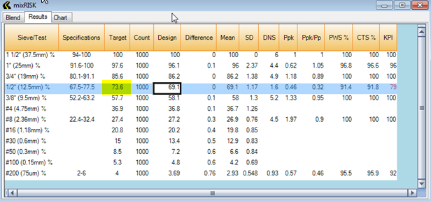
Now it is time to run the Mix Risk tool to assess the variability of each component for the purpose of evaluating the risk of the mix being produced as non-conforming to specifications. As previously mentioned Mix Risk will create a set of randomly generated gradations using the mean and standard deviations for each component and combine them using the percent each is contributing to the design. It is typical to have Mix Risk generate several hundred or a thousand plausible blends. The results of a Mix Risk analysis are shown in Figure 3. It is a good idea to scan the KPI column for low KPI values, generally values below 90 or 95.
 |
| Figure 3. |
In this case, the ½” sieve shows a KPI of 79 and therefore warrants a closer look. Note that the ½” sieve Ppk column shows a value of 0.46, which is below the 0.67 threshold indicating the generated mean value of 69.1 is less than 2 standard deviations away from the closest specification boundary (67.5). The Ppk/Pp value indicates that the mean is significantly off-center in regards to the specification limits. As we discussed in the previous blog that explained the Stonemont KPI, being less than 2 standard deviations away from the closest specification boundary can increase the risk of producing non-conforming material and therefore lower the percent within specification (PWS) value that is routinely used as a basis for pay factors. The conformance to specification (CTS) and PWS values are quite similar and this should be expected from the Mix Risk tool as these gradations are mathematically generated and it is a large sample size. A comparison between CTS and PWS is most useful on production sampling results.
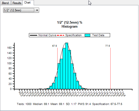
One of the most useful parts of the Mix Risk Analysis is the ability to easily navigate between histograms to review the randomly generated distribution for each sieve size in the mix. The histogram for the ½” sieve is shown in Figure 4. You will notice that the left-tail of the distribution is outside of the lower specification, which is a visual representation of non-conforming results.
 |
| Figure 4. |
Based on these results, we now understand that we have an increased risk of producing non-conforming material due to the ½” sieve size. If we look closely at the ½” sieve, we will notice that the simulated standard deviation is a very reasonable 1.17, which indicates that the mean value of the material is too close to the specification boundary. If this is a new mix the aggregate blend should be modified to try and shift the final result on the ½” sieve to be greater than say 2.5% from the lower specification boundary of 67.5 to reduce the risk of non-conformance. If this is an existing mix one may want to investigate the cause of the mean shift away from the mix JMF. Although Mix Risk identified a potential or possibility for increased risk of producing non-conforming material, it doesn’t indicate that this mix won’t perform well or that non-conforming material will even be produced. It does however give you some potential insight to the possible costs of accepting this increases risk because you may be able to use the simulated PWS and perform a hypothetical pay factor calculation. This may help better understand the risk in terms of cost.
James Beal
Adrian Field
Adrian Field
Stonemont Solutions, Inc.